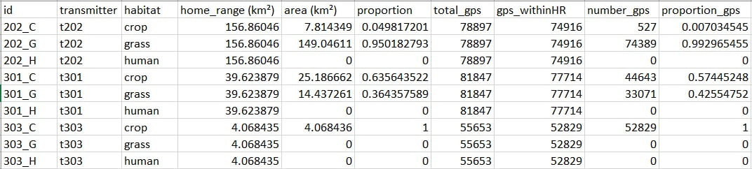
Table 1 represents a subset (n=3) of the total dataset (n=12) used for this project's analysis. Individual ferruginous hawks were assigned an ID using their transmitter number (found in column "transmitter") and treatment (in this case, habitat type). 'C' stands for cropland, 'G' for grassland, and 'H' for human development. The "habitat" column specifies which habitat type (or 'treatment') is measured. The column “home_range (km²)” is the area, measured in km², where 95% of telemetry data points were found for each hawk. The "area (km²)" column is the area, in km², of the habitat type within the home range, and column "proportion" is the proportion of the home range that the habitat occupies. Columns "total_gps" and "gps_withinHR" contain data on the total number of GPS points taken and the number of GPS points found within the 95% home range, respectively. "number_gps" is the number of GPS points in the home range within the specified habitat type, and therefore, "proportion_gps" is the proportion of GPS points found in each habitat type within the home range.
Table 1. Subset (n= 3) of the simplified data table used in R analysis. The ID for each hawk is their transmitter number ("transmitter") and the habitat type (or 'treatment') being measured - 'C' for cropland, 'G' for grassland, and 'H' for human development."home_range" is the total 95% home range of each individual hawk in km², whereas "area" is the area within that home range of that specific habitat type. "proportion" is the proportions of that habitat type of the individual hawk's 95% home range. "total_gps" are the total number of GPS points for the individual hawk's breeding seasons, "gps_withinHR" are the number of GPS points found in the 95% home range, and "number_gps" and "proportion_gps" are the number and proportion of GPS points in each habitat type. Total sample size is n= 12.
The predictor variables in this study and habitat types, whereas the response variable is the proportion of each habitat type within hawk home ranges. The categorical predictor variables, habitat types, were only observed, as large-scale habitat manipulation would not be cost or time effective for this study.
To check my data for errors, I calculated the area of each habitat type, summed these areas, and compared it to the total home range area. Home ranges with habitat types that were not included in the analysis did not have equal area sizes using this comparison, but this was resolved by calculating the areas of the miscellaneous habitat types within the plot to ensure the total home range area was accounted for. This was completed in ArcMap.
Using RStudio, I tested for normality of my habitat proportions and GPS proportions data separately, using both residual plots as well as the Shapiro-Wilk’s test. While my habitat proportion data has a right skew, likely due to the higher values of crop and grassland within home ranges, my use, or GPS, data appeared to have a binomial distribution. I attempted to perform data transformations, however, neither a square root, logistic, or inverse correction with a correction constant to ensure all values were greater than 1 made my data more normal; rather, it caused my habitat proportion data to either maintain a right skew, or turn more binomial. The same pattern was found with my use data. I believe this is because my relatively few categorical habitat ‘treatments’ did not allow for true spread of my data, as human development was so limited, and grassland and cropland had such similar home range proportions and use. As this is a sample of the total population of ferruginous hawks, I decided to use my original data in my statistical analysis, as the transformed data had the same results.
I also checked my proportion data for errors using the summary() function, ensuring that the maximum proportion was one (100%) and that the rest of my minimum and maximum values were properly entered. I found that the mean home range was 198.9 km² (sd=431.5), which was likely increased by the large size of Bird 804’s home range (1594.2 km²). Removing Bird 804 resulted in a mean home range size of 72.0 km² (sd= 67.4). Bird 804 has not successfully nested since the removal of his nest in the winter of 2018, so his large home range size is indicative of many ‘ranging flights’, rather than hunting close to the nest to minimize flight time with prey.
As seen in Figure 10, cropland appears to be the predominant habitat type in Bird 591’s home range, and this pattern appears to be similar for other individuals. There appeared to be similar proportions of grassland and cropland among individual home ranges (Figure 11), as well as a similar pattern in use of the landscape, where grassland and cropland are used at relatively similar rates (Figure 12). No error bars were used as there was not a comparison between multiple treatments or individuals for this graph.

Figure 10. Map of Bird 591's home range. Analysis of this home range can be seen in Figure 11.
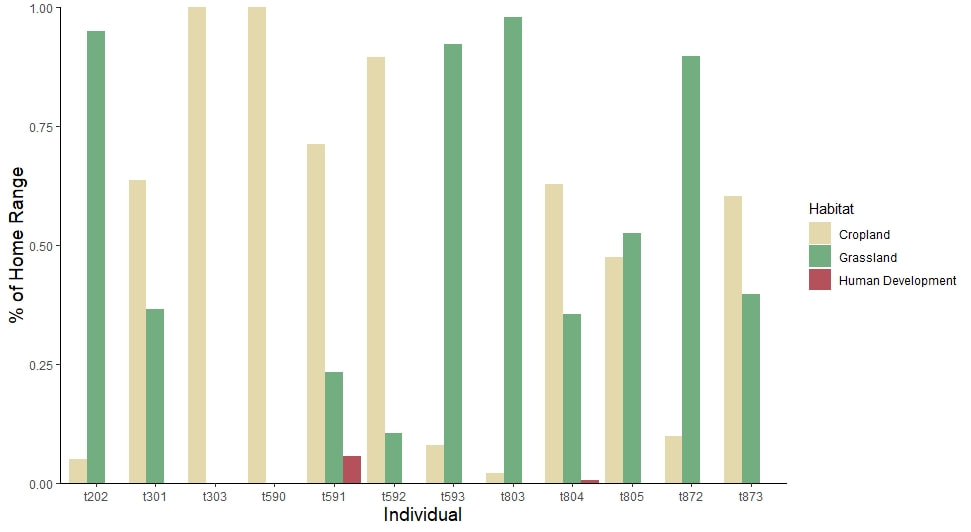
Figure 11. Bar graph representing the proportion of cropland, grassland, and human development in the home range of each individual ferruginous hawk (n=12). Individual hawks are denoted by their transmitter number (eg. t202 = bird with transmitter 202). Habitat type is represented by differing colours, and the % of home range on the y-axis visualizes the proportion of each habitat type within the home range.
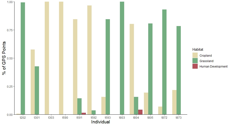
Figure 12. Bar graph representing the proportion of GPS points within an individual hawk's home range by habitat type (n=12). Individual hawks are denoted by their transmitter number (eg. t202 = bird with transmitter 202). Habitat type is represented by differing colours, and the % of GPS points on the y-axis visualizes the proportion of GPS points found in each habitat type, in other words the use of that habitat type, within that hawk's home range.
